- Have Revised
Bio-Potentials
Bio-potentials are important because our bodies inherently have electrically excitable cells. This means they generate potentials (similar to voltage potentials) which can measure for various purposes.
For example:
- ECG - measures our heart
- EMG - measures contracting of muscles
- EEG - Brain behaviour
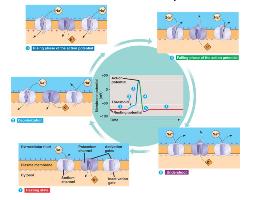
Action-Potentials
So let’s return and have a look at where these action-potentials originate (See L2 for more detail):
- The cell is surrounded by sodium, potassium and chlorine ions.
- Current flow due to movement of Sodium and Potassium ions
- There are more potassium ions inside the cell
- There are more sodium ions outside the cell
- This imbalance sets up a nernst potential, or the imbalance of charge (See L2)
We can think of the lipid membrane almost like a capacitor, because inside the cell it’s full of enriched intracellular potassium ions and outside of the cell, enriched extracellular sodium ions. This insulating membrane with different charges constitutes a potential difference or EMF.
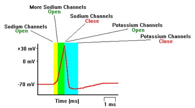
Here you can see the action / generation of this spike visually:
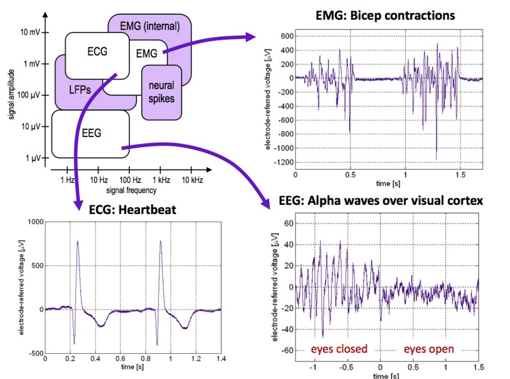
We have seen already the ranges of freq and signal strength of different biopotentials and now we will explore them in greater detail, for example [their morphologies][#sigmorph]
ECG
Our heart pumps due to the rhythmic electrical activity to circulate oxygenated around our body. It all starts in the atrium and then our through the ventricles. We get an initial sinusoidal boom which resonates down into the rest of the heart, providing a superposition kind of effect, we can see this here in the final waveform.
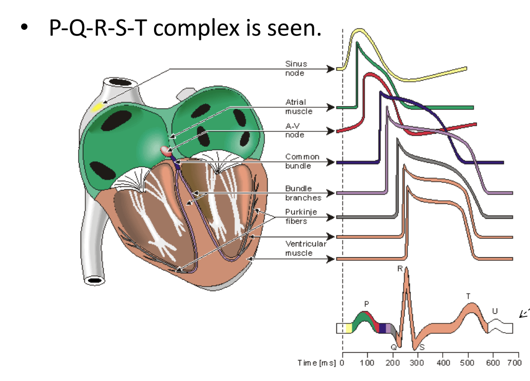
This is described as the PQRST(U) complex
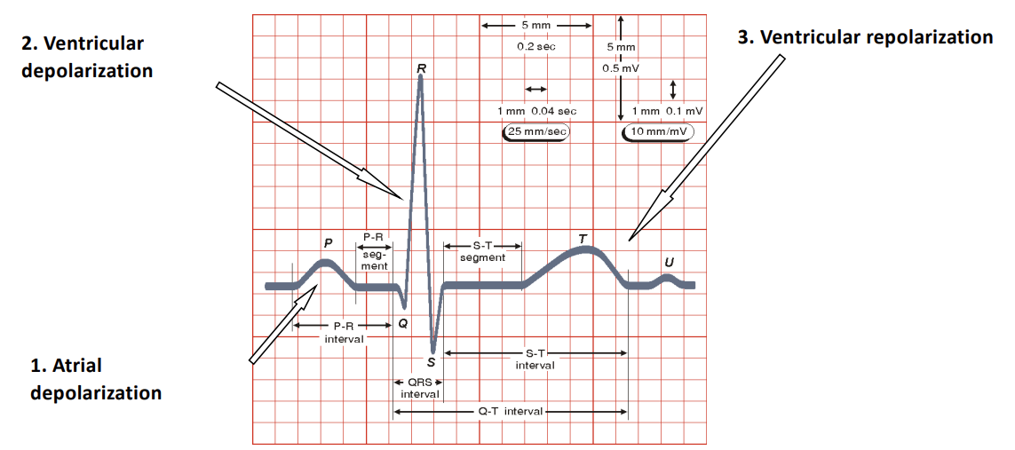
PQRST Complex
So the PQRST complex refers to the characteristic waveform seen on an ECG, representing the electrical activity of the heart’s beat.
- P-Wave
- Reflects the atrial depolarisation which is the electrical activity that causes the atria to contract
- This pushes blood from the atria into the ventricles
- This shows up as a small, rounded upward deflection on the ECG
- QRS Complex
- Reflects the ventricular depolarisation, which is the electrical acitvity that triggers the ventricles to contract
- This pumps blood from ventricles to the lungs
- The ECG shows a small downward deflection (Q-Wave), a sharp tall upward deflection (R-Wave) and a small downward deflection (S-Wave)
- T-Wave
- Reflects the ventricular repolarisation which is the process of ventricles returning to their resting electrical state after contraction
- This shows the muscle relaxing
- This shows up as a broad, rounded upward deflection
- U-Wave (Optional)
- Reflects the repolarisation of the Purkinje fibres
- Is only sometimes present
- Appears as a small , rounded wave following the T-Wave
P-Q, Q-R-S, S-T segments are commonly used for diagnosis.
Measuring ECG
So how do we measure an ECG?
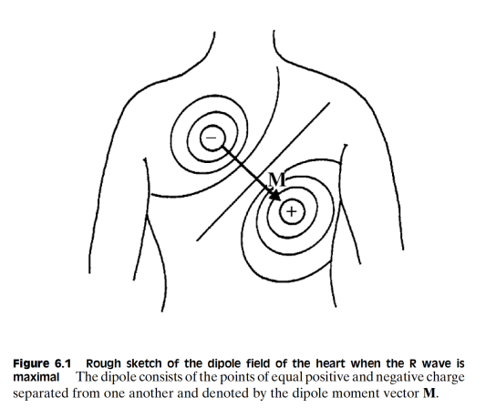
Well given that this is an electrical process, it should be of no suprise that this generates an electric field. This allows us therefore to connect 2 electrodes in the local proximity of the heart to pick up this electric field.
We can characterise this as the cardiac vector
ECG Basics
| Feature | Description |
|---|---|
| Amplitude | 1-5 mV |
| Bandwidth | 0.05-100 Hz |
Largest measurement error sources:
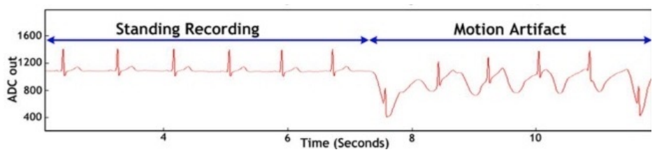
- Motion artifacts (electrodes generated from skin movement)
- 50/60 Hz powerline interference
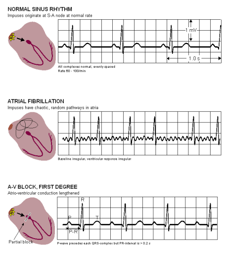
ECG has several applications such as diagnosis of ischemia (lack of blood flow), Arrhythmia (pre-cursor to heart attack), Conduction defects.
EEG
EEG measures the brain electric activity from the scalp, the measured signal results from the activity of billions of neurons. This is broken into various frequency bands for Beta, Alpha, Theta and Delta waves, these can be seen here.
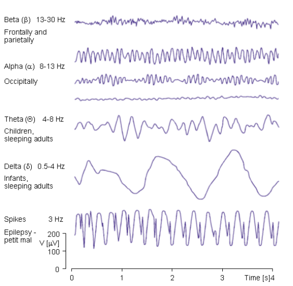
So these constituent bands can tell us varying things, for example Theta waves can be used to determine whether someone is sleeping, they have their eyes open or closed, etc...
| Feature | Description |
|---|---|
| Amplitude | 0.001-0.01 mV |
| Bandwidth | 0.5-40 Hz |
EEG is typically used to study sleep, detect seizures and perform cortical mappings (identification and localisation of functional areas within the cerebral cortex).
EMG
EMG measures the electric activity of active muscle fibres. Electrodes are always connected very close to the muscle group being measured. The rectified and integrated EMG signals gives rough indication of the muscle activity.
| Feature | Description |
|---|---|
| Amplitude | 1-10 mV |
| Bandwidth | 20-2000 Hz |
Errors can occur with regards to 50/60 Hz and RF interference as well as motion artifacts (similar to ECG because we measure from the skin).
The applications of EMG include: Observing muscle function, neuromuscular disease and prosthesis.
Other Bio-Potentials
We also have some other bio-potentials that are touched on in this course:
- Neural Spikes
These are directly monitored from individual neurons in the brain through an implanted microelectrode array
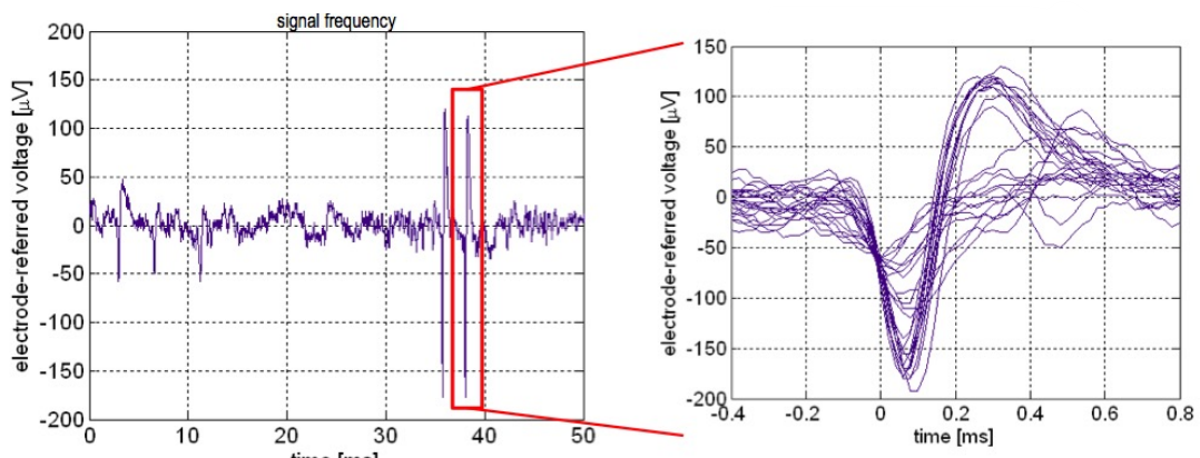
You can see from these graphs that we see a similar action potential, with an extremely small signal amplitude in the micro volts.
- LFP
Local field potentials is the average DC baseline activity measured from an implanted microelectrode. So essentially a measurement of constant activity. This is measured directly on top of the brain using an implant.
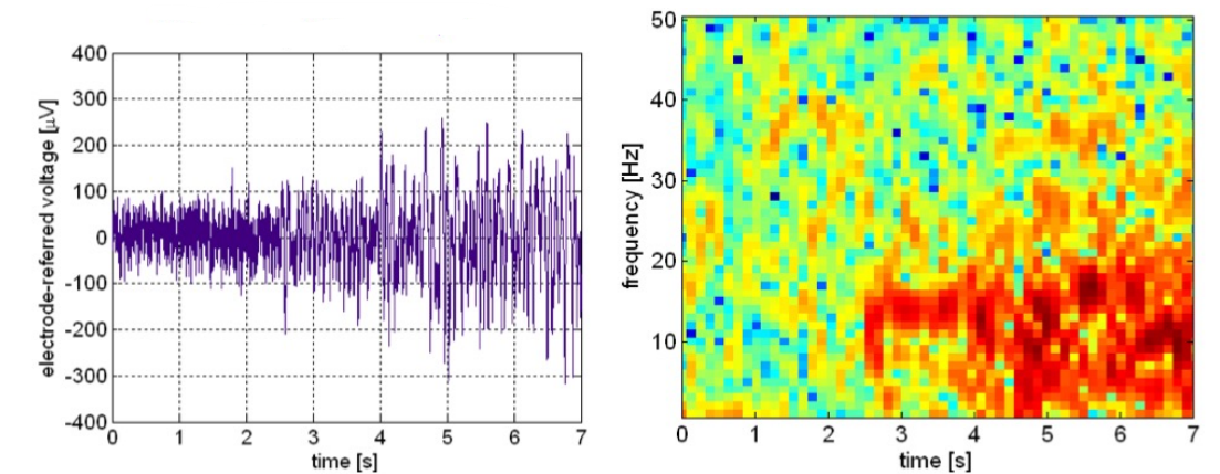
These graphs are examples of LFP recordings, the red on the right might signify that an epileptic seizure is happening in the brain.
Designing and Measuring for Bio-Potentials
So now we’ve covered the basics of the bio-potentials we will be looking at, below is a summary of all the signals and their descriptions.
| Signal | Freq Range (Hz) | Amplitude range (mV) |
|---|---|---|
| ECG | 0.05-100 | 1-5 |
| EEG | 0.5-40 | 0.001 - 0.01 |
| EMG | 20-2000 | 1-10 |
| Neural Spikes | 300-5000 | 0.001 - 0.5 |
| Local Field Potentials | 10-200 | 0.001 - 5 |
In order to measure bio-potentials we generally need to use contacts on the body, like an electrode. This signal then goes into an amplifier, which measures the potential and then it goes onto a filter of some kind. This has to be robust as to avoid noise.
This amplifier is very important and we need to consider some requirements:
- High I/P Impedance - so as not to attenuate the measured signal
- High Gain & Low Noise - to detect and amplify very small signals
- High CMRR - to discard common noise to both terminals, such as 50 Hz noise
- Band Pass Filtering - to select the frequency range of interest
Recall CMRR
CMMR is the ability of the amplifier to discard signals which are common to both terminals. In this case you’ll have 50/60 Hz noise common to both terminals, so it should reject it.
The general architecture of an ECG measurement system is as follows, this is really important:
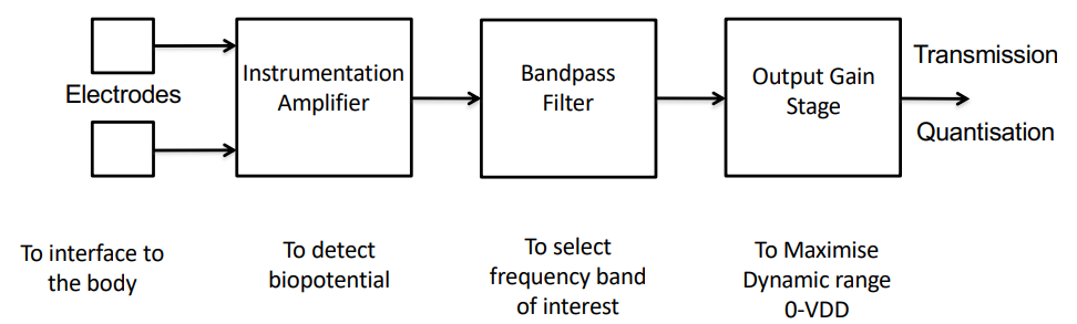
Considerations for Detection
Before going into depth on each component of the architecture, let’s see the things we should be considering when designing our systems:
- High input impedance (> 50MΩ)
- Gain (> 40dB)
- High CMRR (> 70dB)
- Resolution – 6-12 Bits (depending on application)
- Noise – signal dependent, typically < 10uV RMS
- Frequency – signal dependent, typically < 10 KHz
- Power consumption – application dependent
- Interfering inputs – mains noise, electrode impedance, offset.
- Placement of Electrodes – Distance, intracellular, extracellular.
Electrodes
So let’s start by looking at the main interface to the tissue, electrodes.
Electrodes are basically conductive to the skin, they can be silver (usually in a saline solution to enhance the conductive layer) or also implantable. These implantable ones usually go directly into the brain where as the skin surface electrodes are generally for ECG, EMG and EEG.
Electrode grids for recording for the brain surface is called ECoG. This generally measures low-frequency EEG/LFP-like signals (individual neurons not observable)
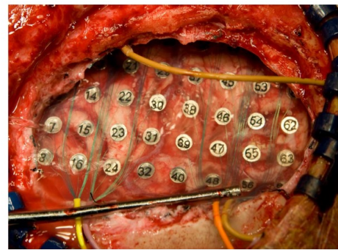
This is used to identify and localise areas of the brains causing seizures.
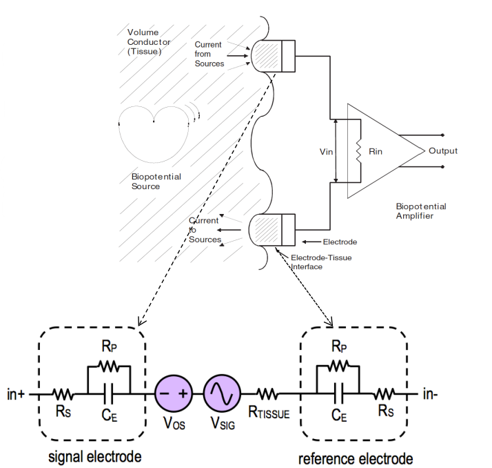
Something we need to be very mindful of is the impedance consideration between the surface of the skin and the actual signal source we are measuring. We can approximate this to a resistor capacitor network.
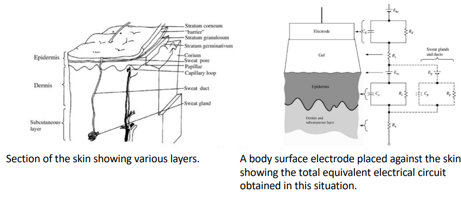
This is something we need to consider when making our instrumentation. This is a reasonably equivalent circuit model that we use for the electrode tissue interface.
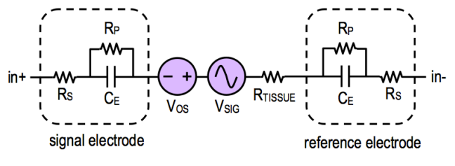
Where:
- : capacitance of electrode-electrolyte interface
- : resistance of electrode-electrolyte interface
- : resistance of electrode lead wire
- : resistance of tissue
- : detected bio-potential
- : common mode offset
We need measuring instruments to have higher impedance than electrode impedance so as not to attenuate the signal (we also need small input capacitance).
When designing we can treat the electrode-instrumentation interface as a simple RC circuit on the I/P of the amplifier.
Impedance Levels
We want input impedance to be very high so that it doesn’t divide down your I/P signal. So it doesn’t divert any current from the I/P to itself even if the input has very high resistance (e.g an opamp taking I/P from microelectrode)
Our output impedance should be very low, so that we can drop the maximum voltage over the next stage load. So it can supply output even to very low resistive loads and not expend most of it on itself.
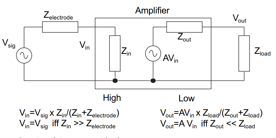
We note from the maths in this diagram that the input resistance must be huge and the input capacitance of the amplifier must be small relative to the electrode.
Noise
Mains 50Hz Noise
So let’s look a bit at noise, starting from the mains 50Hz noise.
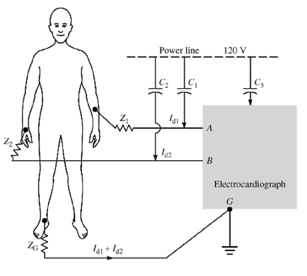
Here we see that the wire connecting the electrodes to the instrumentation are also passively coupled to the power line via capacitors and . The net result of that is it will cause a small current to flow ( and ).
This current flows through the skin-electrode impedances and , this can be modelled like so:
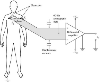
Common Mode Noise
Another source of noise is common mode noise.
So if we get rid of the wires and integrate the circuit like a patch, current couples from the power line through and flows through the body and ground impedance
This causes a common mode voltage everywhere in the body ()
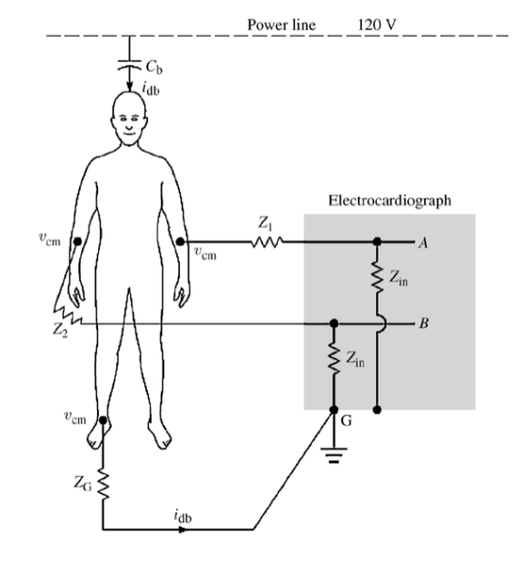
The induced noise on measured voltage is given as a consistent offset:
Typically = 0.2uA x 50kΩ = 10mV.
Normally common mode noise would be rejected by amplifiers, however finite input impedance of the amplifier and different impedance in leads and can cause a slight offset to appear:
Motion Artifacts
If a pair of electrodes is in an electrolyte and one moves with respect to the other, a potential difference appears across the electrodes known as the motion artifact.
This is a source of noise and interference in biopotential measurements. It is a result of the change in distribution of the double layer of charge on the polarizable electrode interface because of movement. This changes the half cell potential of the electrode temporarily.
Solutions
| Type of Noise | Solution |
|---|---|
| 50 Hz power lines | shielding, filtering |
| Other biopotentials | filtering |
| Motion artifacts | relaxed subject, signal processing |
| Electrode noise | high quality electrodes, good contacts |
| Circuit noise | good design, good components |
| Common mode noise | differential design, high CMRR |
Biopotential Amplifier
We will now proceed in designing some bio-potential amplifiers, but first we have some requirements.
An integrated front-end amplifier for bio-potentials should:
Amplify signals in the frequency bands of interest;
Block dc offsets present at the electrode-tissue interface to prevent saturation of the amplifier;
Have sufficiently low input-referred noise to resolve biological signals in the low microvolt range;
Have sufficient dynamic range to convey signals in the low millivoltrange;
Have much higher input impedance than the electrode-tissue interface and have negligible dc input current;
Reject common-mode signals (high CMRR) particularly at 50/60 Hz; reject power supply noise (high PSRR);
Consume little power, to facilitate wearable or implantable applications.
Instrumentation Amplifier
So we need to make an amplifier to set the voltage, the easiest amplifier we know is an opamp in a closed loop configuration.
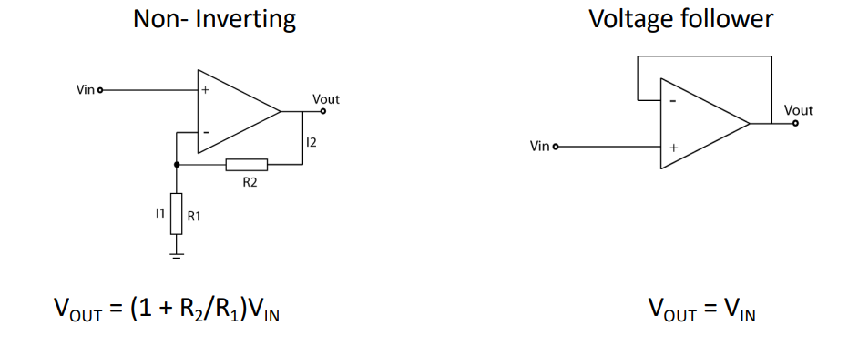
This can give us the gain we need however it lacks immunity to common mode signals. So our 50Hz noise will be amplified. So how do we get rid of this problem?
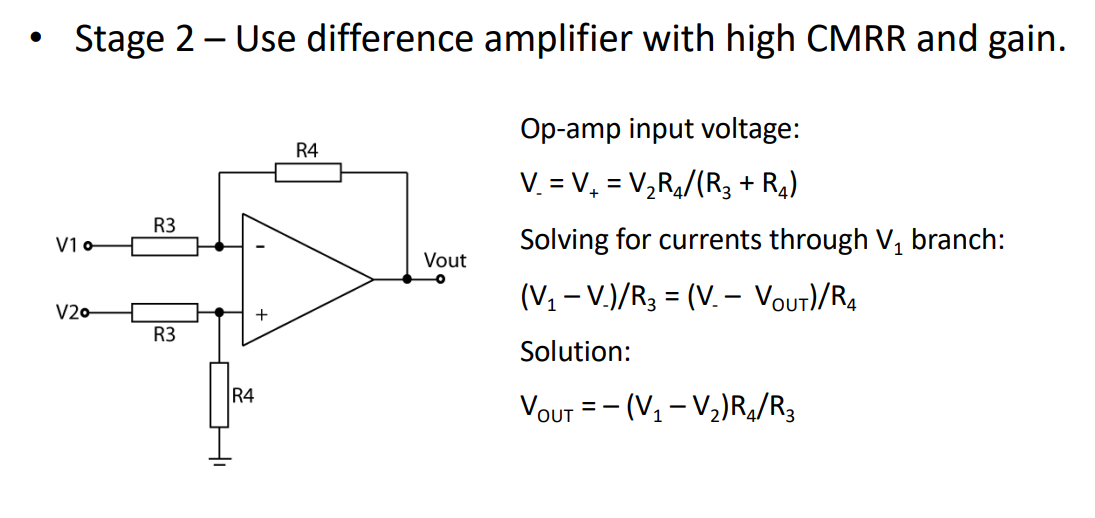
We can use a difference amplifier. These are good for rejecting common mode signals, so we don’t have to worry about the 50Hz noise.
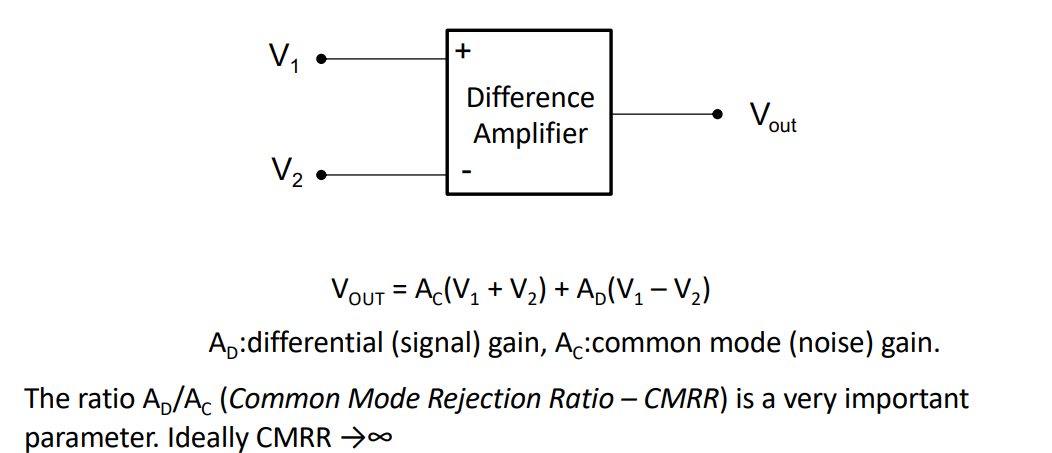
This amplifies the difference between and but rejects any common mode signals.
Differential Instrumentation Amplifier 1
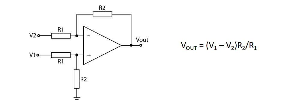
In this case:
So CMRR is infinite! However this is assuming the resistors are matched, and mismatch seriously degrades CMRR, and therefore not infinite in the real world. Also input impedance is not infinite, it’s set by !
Differential Instrumentation Amplifier 2
So how do we fix this? Well let’s stick another stage in front of it which has a really high I/P impedance:
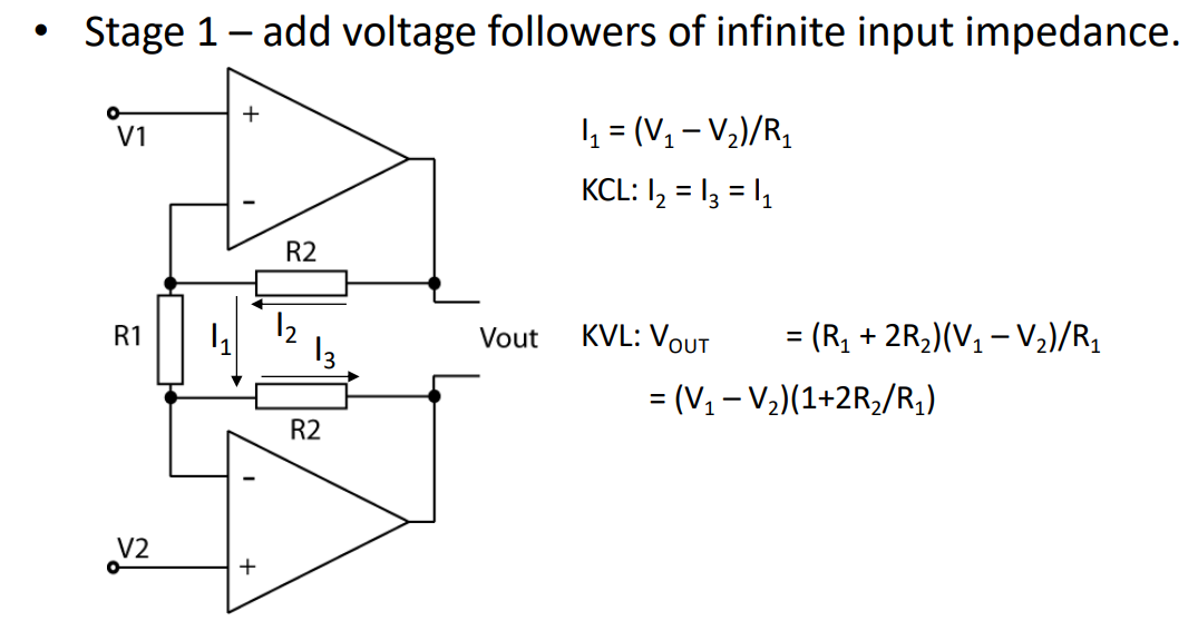
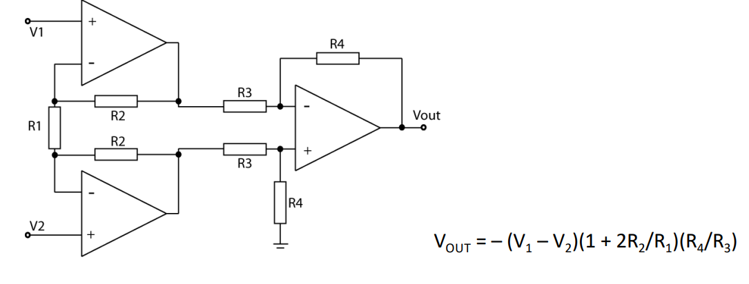
So now we have really high I/P impedance from the opamps, we can then add this back to the previous circuit.
Giving us our final diagram. This now has a high I/P impedance and high CMRR. The gain is normally tuned by a variable resistor in place of .
Electrical Interference Reduction
What can we do to reject 50/60 Hz noise?
Common mode interference would be completely rejected by the instrumentation amplifier if the matching were ideal, however this is often not the case. A clever trick is the “driven right leg circuit”, which works to enhance the CMRR for ECG.
The idea being the Average of the is inverted and driven back to the body via a reference electrode
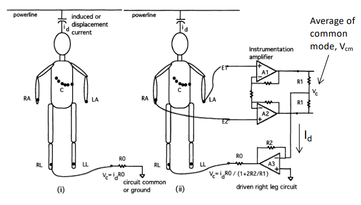
Right Leg Drive Circuit
Through feedback the body’s displacement current flows not to instrument ground but to the O/P of the opamp. This reduces :
if we recall without the driven right leg circuit which has now been reduced by ratio of resistors and . The circuit also provides electrical safety as the maximum current is limited by the feedback opamp.
Filtering
What we’ve covered so far is on the front end, now we need to consider that different bio-potential signals occupy certain frequency ranges. This means we need a BPF to select only the range we want.
To do this we can cascade a HPF and a LPF
NOTE: We also describe the cut off frequency at the 3dB point, when the I/P signal is attenuated of half the power
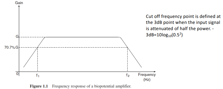
We can use spectral analysis of the signal to determine the bandwidth. An estimate can also be derived by looking at the durations of the low and high frequency components of the signal.
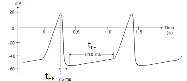
- High Frequency: is the minimum rise or fall time of the signal
- Low Frequency: is the tilt of the baseline or lowest frequency component
Filter Response Laplace
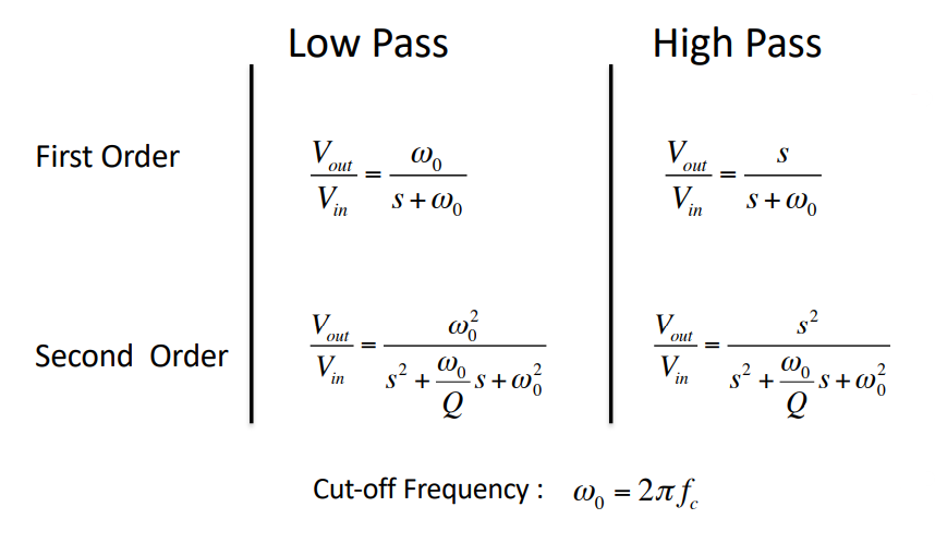
factor : Determines the height and width of the peak of the frequency response of the filter
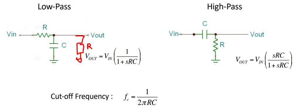
RC Filter
The RC filter has no active components, only passive. Therefore they require no power supply and there’s no gain attenuation. However there is no buffering or high I/P impedance.
To prevent loading we add a voltage buffer op-amp between stages
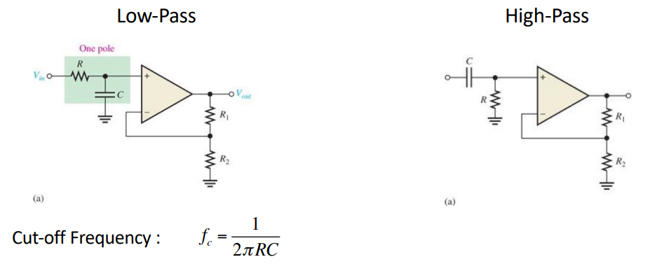
Op-Amp Filter
This is an active filter which can also amplify the signal (with a gain of ). This also does not do loading of successive stages. Unfortunately this is limited by the op-amp’s frequency response.
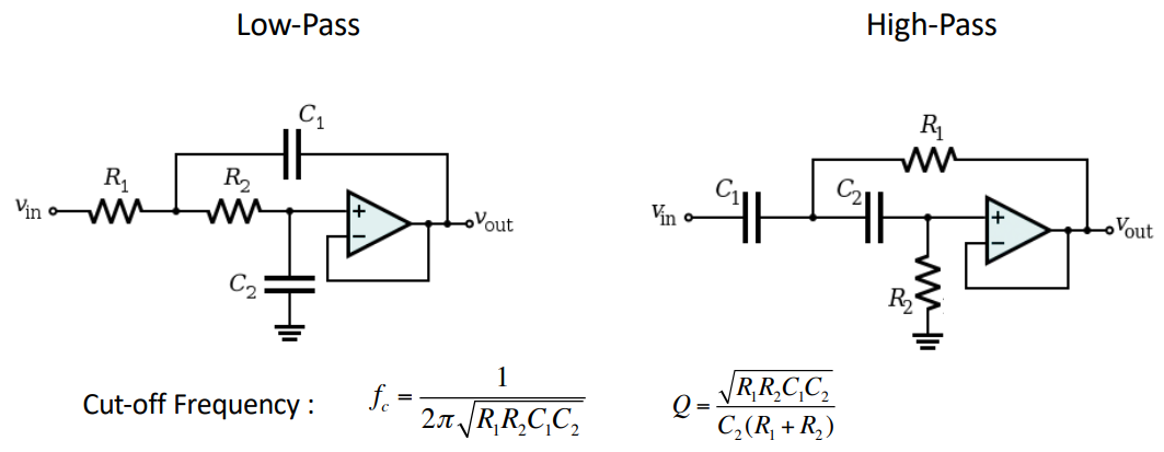
Sallen-Key Filter
These are relatively simple circuits which can realise 2nd order filters with a single op-amp. If we cascade these we can make brick wall filters.
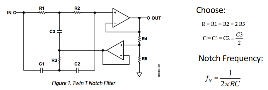
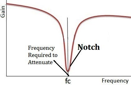
Notch Filter
These directly filter out 50/60Hz noise. BUT be careful that you don’t filter out vital information if it is within the frequency bandwidth, therefore it’s best to use only when you absolutely have to.
Final ECG
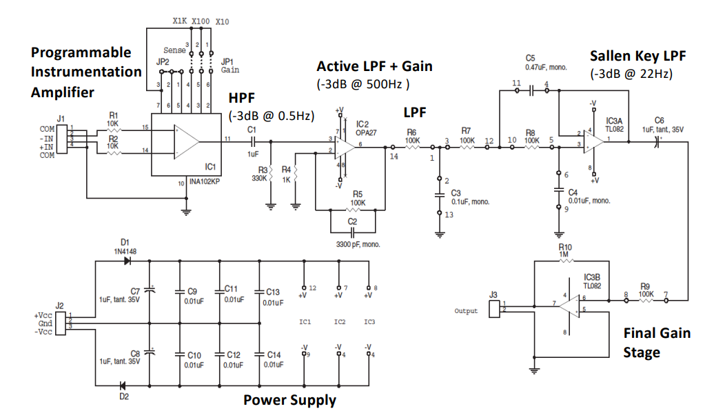
AC Coupled Bio-Potential Amplifiers
For very small Bio-potentials in the mV range we need a really high gain at the I/P stage. This is why we need AC coupled Bio-Potential amplifiers, which only let AC go to the amplifier at the 1st stage.
The idea is that DC offset voltage on I/P can be so large that it saturates the amplifier, this makes it difficult to add lots of gain in front-end. The solution is to capacitvely couple
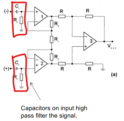
There are some problems with this method:
- This can degrade CMRR due to poor matching of components.
- Input capacitance must be smaller than electrode capacitance otherwise there will be attenuation.
- Charging currents can cause undefined voltages on the input, thus need to add resistor to fix the input DC voltage.
- This reduces the input impedance significantly.
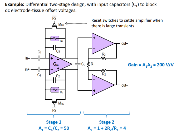
The Harrison Amplifier
The Harrison Amplifier is an example of a state of the art AC coupled instrumentation amplifier.
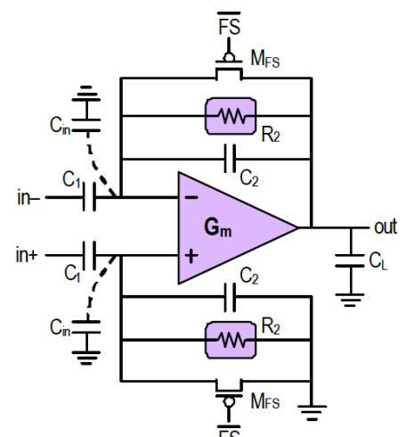
Need to ensure that is smaller then electrode capacitance so signal is not attenuated AND resistor is required to set the common mode I/P of the amplifier.
Below is the complete TF, don’t worry you don’t have to derive:
This network of capacitors and resistors produce a frequency response of a BPF as well.
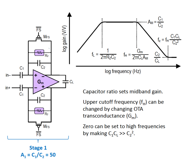
And we can also add a 2nd amplification stage